Filters: Tags: scenarios (X)
122 results (36ms)|
Filters
Contacts
(Less)
|
Spatially-explicit state-and-transition simulation models of land use and land cover (LULC) increase our ability to assess regional landscape characteristics and associated carbon dynamics across multiple scenarios. By characterizing appropriate spatial attributes such as forest age and land-use distribution, a state-and-transition model can more effectively simulate the pattern and spread of LULC changes. This manuscript describes the methods and input parameters of the Land Use and Carbon Scenario Simulator (LUCAS), a customized state-and-transition simulation model utilized to assess the relative impacts of LULC on carbon stocks for the conterminous U.S. The methods and input parameters are spatially explicit...
Categories: Publication;
Types: Journal Citation;
Tags: Land use and Land cover,
Scenarios,
Spatially-explicit modeling,
State-and-transition simulation model

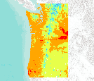
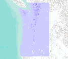
Soil residual water corresponds to the model variable "total streamflow." In the model MC1, this is calculated (in cm of water) as the water flowing through the soil profile below the last soil layer (streamflow), water leached into the subsoil (baseflow) and also includes runoff. The output is presented here as a monthly average. Soil residual water is part of the model output from Brendan Rogers' MS thesis work. Brendan used the vegetation model MC1 to simulate vegetation dynamics, associated carbon and nitrogen cycle, water budget and wild fire impacts across the western 2/3 of the states of Oregon and Washington using climate input data from the PRISM group (Chris Daly, OSU) at a 30arc second (800m) spatial...

Soil residual water corresponds to the model variable "total streamflow." In the model MC1, this is calculated (in cm of water) as the water flowing through the soil profile below the last soil layer (streamflow), water leached into the subsoil (baseflow) and also includes runoff. The output is presented here as a monthly average. Soil residual water is part of the model output from Brendan Rogers' MS thesis work. Brendan used the vegetation model MC1 to simulate vegetation dynamics, associated carbon and nitrogen cycle, water budget and wild fire impacts across the western 2/3 of the states of Oregon and Washington using climate input data from the PRISM group (Chris Daly, OSU) at a 30arc second (800m) spatial...

Soil residual water corresponds to the model variable "total streamflow." In the model MC1, this is calculated (in cm of water) as the water flowing through the soil profile below the last soil layer (streamflow), water leached into the subsoil (baseflow) and also includes runoff. The output is presented here as a monthly average. Soil residual water is part of the model output from Brendan Rogers' MS thesis work. Brendan used the vegetation model MC1 to simulate vegetation dynamics, associated carbon and nitrogen cycle, water budget and wild fire impacts across the western 2/3 of the states of Oregon and Washington using climate input data from the PRISM group (Chris Daly, OSU) at a 30arc second (800m) spatial...

Soil residual water corresponds to the model variable "total streamflow." In the model MC1, this is calculated (in cm of water) as the water flowing through the soil profile below the last soil layer (streamflow), water leached into the subsoil (baseflow) and also includes runoff. The output is presented here as a monthly average. Soil residual water is part of the model output from Brendan Rogers' MS thesis work. Brendan used the vegetation model MC1 to simulate vegetation dynamics, associated carbon and nitrogen cycle, water budget and wild fire impacts across the western 2/3 of the states of Oregon and Washington using climate input data from the PRISM group (Chris Daly, OSU) at a 30arc second (800m) spatial...

Soil residual water corresponds to the model variable "total streamflow." In the model Mc1, this is calculated (in cm of water) as the water flowing through the soil profile below the last soil layer (streamflow), Water leached in the subsoil (baseflow) and also includes runoff. the output is prsented here as a monthly average. Soil residual water is part of the model output from Brendan Rogers' MS thesis work. Brendan used the vegetation model MC1 to simulate vegetation dynamics, associated carbon and nitrogen cycle, water budget and wild fire impacts across the western 2/3 of the states of Oregon and Washington using climate input data from the PRISM group (Chris Daly, OSU) at a 30arc second (800m) spatial grain....
Improving energy efficiency is the most effective and least expensive way to reduce carbon dioxide (C02) emissions in most industrialized nations - including the UK. A report from the UKAEA's own Energy Technology Support Unit concludes that energy efficiency can displace nearly four times more C02 than nuclear power can - more quickly and more cost-effectively. Each pound invested in efficient lighting can displace four to five times as much C02 as a pound invested in new nuclear power. Meanwhile, given recent dramatic progress in renewable energy technologies, the most promising long-term COz-abatement strategy may be a synergistic combination of energy efficiency and renewable energy.
Categories: Publication;
Types: Citation;
Tags: Effort,
climate change,
global,
mitigation,
scenarios
Our responses to the emerging challenges of energy planning have to be faster and more effective than they have been so far. While the Gulf war has forced us to realise the danger, it is to be hoped that the solutions that are sought will take the form not of short-term palliatives but of a new direction in our planning effort. Sixth of a series of articles discussing the broad approach of the Planning Commission under the V P Singh government.
Categories: Publication;
Types: Citation;
Tags: Effort,
climate change,
global,
mitigation,
scenarios
For his MS thesis, Brendan Rogers used climate data from the PRISM group (Chris Daly, Oregon State University) at a 30arc second (800m) spatial grain across the western 2/3 of the states of Oregon and Washington to generate a climatology or baseline. He then created future climate change scenarios using statistical downscaling to create anomalies from three General Circulation Models (CSIRO Mk3, MIROC 3.2 medres, and Hadley CM 3), each run through three CO2 emission scenarios (SRES B1, A1B, and A2).

For his MS thesis, Brendan Rogers used climate data from the PRISM group (Chris Daly, Oregon State University) at a 30arc second (800m) spatial grain across the western 2/3 of the states of Oregon and Washington to generate a climatology or baseline. He then created future climate change scenarios using statistical downscaling to create anomalies from three General Circulation Models (CSIRO Mk3, MIROC 3.2 medres, and Hadley CM 3), each run through three CO2 emission scenarios (SRES B1, A1B, and A2).

For his MS thesis, Brendan Rogers used climate data from the PRISM group (Chris Daly, Oregon State University) at a 30arc second (800m) spatial grain across the western 2/3 of the states of Oregon and Washington to generate a climatology or baseline. He then created future climate change scenarios using statistical downscaling to create anomalies from three General Circulation Models (CSIRO Mk3, MIROC 3.2 medres, and Hadley CM 3), each run through three CO2 emission scenarios (SRES B1, A1B, and A2).
For his MS thesis, Brendan Rogers used the vegetation model MC1 to simulate vegetation dynamics, associated carbon and nitrogen cycle, water budget and wild fire impacts across the western 2/3 of the states of Oregon and Washington using climate input data from the PRISM group (Chris Daly, OSU) at a 30arc second (800m) spatial grain. The model was run from 1895 to 2100 assuming that nitrogen demand from the plants was always met so that the nitrogen concentrations in various plant parts never dropped below their minimum reported values. A CO2 enhancement effect increased productivity and water use efficiency as the atmospheric CO2 concentration increased. Future climate change scenarios were generated through statistical...
For his MS thesis, Brendan Rogers used the vegetation model MC1 to simulate vegetation dynamics, associated carbon and nitrogen cycle, water budget and wild fire impacts across the western 2/3 of the states of Oregon and Washington using climate input data from the PRISM group (Chris Daly, OSU) at a 30arc second (800m) spatial grain. The model was run from 1895 to 2100 assuming that nitrogen demand from the plants was always met so that the nitrogen concentrations in various plant parts never dropped below their minimum reported values. A CO2 enhancement effect increased productivity and water use efficiency as the atmospheric CO2 concentration increased. Future climate change scenarios were generated through statistical...
This project assessed the potential effects of climate change on tidal marsh habitats and bird populations, identified priority sites for tidal marsh conservation and restoration, and developed a web-based mapping tool for managers to interactively display and query results. Project results can be found at PRBO’s San Francisco Bay Sea-Level Rise Website
Categories: Data,
Project;
Tags: 2010,
2013,
Applications and Tools,
CA,
California Landscape Conservation Cooperative,
Phase 1 & 2 (2010, 2012): This project developed a sampling design and monitoring protocol for wintering shorebirds in the Central Valley and in the San Francisco Bay Estuary and develop an LCC-specific online shorebird monitoring portal publicly available at the California Avian Data Center. The three objectives in Phase II of this project are: 1) Complete the shorebird monitoring plan for the CA LCC by developing a sampling design and monitoring protocol for wintering shorebirds in coastal southern California and northern Mexico. 2) Develop models to evaluate the influence of habitat factors from multiple spatial scales on shorebird use of San Francisco Bay and managed wetlands in the Sacramento Valley, as a model...
Categories: Data,
Project;
Types: Map Service,
OGC WFS Layer,
OGC WMS Layer,
OGC WMS Service;
Tags: 2010,
2011,
2013,
Academics & scientific researchers,
Academics & scientific researchers,
The Chernobyl accident was a major economic loss with a cost of about $12.5 billion U.S. dollars to the government of the Soviet Union. However, in terms of human loss it was less than a major accident. The economic costs in countries other than the Soviet Union were caused by reasons other than established radiation protection principles. The lack of preparedness of most countires was demonstrated by exaggerated reporting by the news media and by the confused actions of governments.

For his MS thesis, Brendan Rogers used climate data from the PRISM group (Chris Daly, Oregon State University) at a 30arc second (800m) spatial grain across the western 2/3 of the states of Oregon and Washington to generate a climatology or baseline. He then created future climate change scenarios using statistical downscaling to create anomalies from three General Circulation Models (CSIRO Mk3, MIROC 3.2 medres, and Hadley CM 3), each run through three CO2 emission scenarios (SRES B1, A1B, and A2).
In response to the increasing global demand for energy, on exploration and development are expanding into frontier areas of the Arctic, where slow-growing tundra vegetation and the underlying permafrost Soils are Very sensitive to disturbance. The creation of vehicle trails on the tundra from seismic exploration for on has accelerated in the past decade, and the cumulative impact represents a geographic footprint that covers a greater extent of Alaska's North Slope tundra than all other direct human impacts combined. Seismic exploration for on and gas was conducted on the coastal plain of the Arctic National Wildlife Refuge, Alaska, USA, in the winters of 1984 and 1985. This study documents recovery Of vegetation...
Categories: Publication;
Types: Citation;
Tags: Implementation,
carbon,
challenges,
fuel,
scenarios,
Global land-use/land-cover (LULC) change projections and historical datasets are typically available at coarse grid resolutions and are often incompatible with modeling applications at local to regional scales. The difficulty of downscaling and reapportioning global gridded LULC change projections to regional boundaries is a barrier to the use of these datasets in a state-and-transition simulation model (STSM) framework. Here we compare three downscaling techniques to transform gridded LULC transitions into spatial scales and thematic LULC classes appropriate for use in a regional STSM. For each downscaling approach, Intergovernmental Panel on Climate Change (IPCC) Representative Concentration Pathway (RCP) LULC...
Categories: Publication;
Types: Journal Citation;
Tags: Conterminous United States,
Downscaling,
Land use and Land cover,
RCPs,
Representative Concentration Pathways,
Soil residual water corresponds to the model variable "total streamflow"." In the model MC1, this is calculated (in cm of water) as the water flowing through the soil profile below the last soil layer (streamflow), water leached into the subsoil (baseflow) and also includes runoff. The output is presented here as a monthly average. Soil residual water is part of the model output from Brendan Rogers' MS thesis work. Brendan used the vegetation model MC1 to simulate vegetation dynamics, associated carbon and nitrogen cycle, water budget and wild fire impacts across the western 2/3 of the states of Oregon and Washington using climate input data from the PRISM group (Chris Daly, OSU) at a 30arc second (800m) spatial...
|

|
