Filters: Tags: species (X)
784 results (11ms)|
Filters
Date Range
Extensions
Types
Contacts
Categories
Tag Types
|

The Nature Conservancy (TNC) has derived climate suitability forecasts for most species of trees and shrubs considered to be ecological dominants of terrestrial Californian habitat types. Our plant projections are compiled as decision support tools to help Conservancy project staff, as well as our external partners, develop the necessary plans, priorities and strategies to successfully adapt to uncertain changes in future climate. In the recently completed Southern Sierra Partnership's 2010 Climate-Adapted Conservation Plan for the Southern Sierra Nevada and Tehachapi Mountains, species and habitat forecasts shown here informed the development of a regional conservation design that explicitly incorporates long-term...
The Nature Conservancy (TNC) has derived climate suitability forecasts for most species of trees and shrubs considered to be ecological dominants of terrestrial Californian habitat types. Our plant projections are compiled as decision support tools to help Conservancy project staff, as well as our external partners, develop the necessary plans, priorities and strategies to successfully adapt to uncertain changes in future climate. In the recently completed Southern Sierra Partnership's 2010 Climate-Adapted Conservation Plan for the Southern Sierra Nevada and Tehachapi Mountains, species and habitat forecasts shown here informed the development of a regional conservation design that explicitly incorporates long-term...

The Nature Conservancy (TNC) has derived climate suitability forecasts for most species of trees and shrubs considered to be ecological dominants of terrestrial Californian habitat types. Our plant projections are compiled as decision support tools to help Conservancy project staff, as well as our external partners, develop the necessary plans, priorities and strategies to successfully adapt to uncertain changes in future climate. In the recently completed Southern Sierra Partnership's 2010 Climate-Adapted Conservation Plan for the Southern Sierra Nevada and Tehachapi Mountains, species and habitat forecasts shown here informed the development of a regional conservation design that explicitly incorporates long-term...

These data identify, in general, the areas where final critical habitat for Castilleja cinerea (Ash-gray Indian paintbrush) occur.

Species range maps for Wyoming developed by the Wyoming Natural Diversity Database.
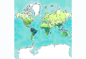
Number of amphibian species, by freshwater ecoregion. We calculated the number of amphibian species per freshwater ecoregion using species range maps of the Global Amphibian Assessment (GAA, www.iucnredlist.org/amphibians) (IUCN et al. 2006). The 2006 GAA assessed 5,918 amphibian species and provided distribution maps for 5,640 of those species. When a range overlapped several ecoregions, we counted species as present in all those ecoregions that had part of the range. This may have resulted in an overestimate of species numbers in some ecoregions, especially those that are long and narrow in shape. This is particularly true for the Amazonas High Andes ecoregion (312), where the mountain range has been used as...

Major forest species of Russia, created from an amalgamation of all applicable IIASA data with the Forest State Account of 1993, produced at a scale of 1:1 million. It is p art of the Land Resources of Russia collection. More information on the forestry datasets can be found at: http://www.iiasa.ac.at/Research/FOR/russia_cd/forestry.htm .

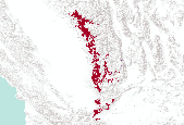
The source of this coverage data set is the fish biodiversity maps created for The Nature Conservancy (TNC) as part of their Hexagon Project. Professor Peter Moyle and his graduate student, Paul Randall, of the Department of Wildlife and Fisheries Conservation Biology at the University of California, Davis were hired to produce range maps for all known fish species that presently occur in California. Each coverage denotes a separate fish species (refer to the species coverage key below). The polygons are estimated to be accurate at a scale of roughly 1:1,000,000. Other California fish species distributions can be found in a gallery at: http://app.databasin.org/app/pages/galleryPage.jsp?id=099b47b7394f47b6b42764829e8a8f09

Species occurrence data were obtained from the Atlas of Spawning and Nursery Areas of Great Lakes Fishes (Goodyear et al. 1982). The atlas contains information on all of the commercially and recreationally important species that use the tributaries, littoral and open-water areas of the Great Lakes as spawning and nursery habitats. Close to 9500 geo-referenced data records (occurrences of fish species) were imported into ArcView GIS. The 139 fish taxa reported in the Atlas had to be grouped into fewer broad categories to produce meaningful distribution maps. We chose three functional classification schemes. Jude and Pappas (1992) used Correspondence Analysis to partition fish species associated with the open...

Species occurrence data were obtained from the Atlas of Spawning and Nursery Areas of Great Lakes Fishes (Goodyear et al. 1982). The atlas contains information on all of the commercially and recreationally important species that use the tributaries, littoral and open-water areas of the Great Lakes as spawning and nursery habitats. Close to 9500 geo-referenced data records (occurrences of fish species) were imported into ArcView GIS. The 139 fish taxa reported in the Atlas had to be grouped into fewer broad categories to produce meaningful distribution maps. We chose three functional classification schemes. Jude and Pappas (1992) used Correspondence Analysis to partition fish species associated with the open...

This dataset represents presence of Jack Pine (Pinus banksiana) in Minnesota (USA) at year 50 (2045) from a single model run of LANDIS-II. The simulation assumed Intergovernmental Panel on Climate Change (IPCC) B2 emissions (moderate) and used the Hadley 3 global circulation model. Restoration harvest rates and intensities were simulated.

This dataset represents presence of Sugar Maple (Acer saccharum) in Minnesota (USA) at year 0 (2145) from a single model run of LANDIS-II. The simulation assumed Intergovernmental Panel on Climate Change (IPCC) B2 emissions (moderate) and used the Hadley 3 global circulation model. Contemporary harvest rates and intensities were simulated.

These data identify, in general, the areas where final critical habitat for Erigeron parishii (Parish's daisy) occur.

The source of this coverage data set is the fish biodiversity maps created for The Nature Conservancy (TNC) as part of their Hexagon Project. Professor Peter Moyle and his graduate student, Paul Randall, of the Department of Wildlife and Fisheries Conservation Biology at the University of California, Davis were hired to produce range maps for all known fish species that presently occur in California. Each coverage denotes a separate fish species (refer to the species coverage key below). The polygons are estimated to be accurate at a scale of roughly 1:1,000,000. Other California fish species distributions can be found in a gallery at: http://app.databasin.org/app/pages/galleryPage.jsp?id=099b47b7394f47b6b42764829e8a8f09

The source of this coverage data set is the fish biodiversity maps created for The Nature Conservancy (TNC) as part of their Hexagon Project. Professor Peter Moyle and his graduate student, Paul Randall, of the Department of Wildlife and Fisheries Conservation Biology at the University of California, Davis were hired to produce range maps for all known fish species that presently occur in California. Each coverage denotes a separate fish species (refer to the species coverage key below). The polygons are estimated to be accurate at a scale of roughly 1:1,000,000. Other California fish species distributions can be found in a gallery at: http://app.databasin.org/app/pages/galleryPage.jsp?id=099b47b7394f47b6b42764829e8a8f09

The source of this coverage data set is the fish biodiversity maps created for The Nature Conservancy (TNC) as part of their Hexagon Project. Professor Peter Moyle and his graduate student, Paul Randall, of the Department of Wildlife and Fisheries Conservation Biology at the University of California, Davis were hired to produce range maps for all known fish species that presently occur in California. Each coverage denotes a separate fish species (refer to the species coverage key below). The polygons are estimated to be accurate at a scale of roughly 1:1,000,000. Other California fish species distributions can be found in a gallery at: http://app.databasin.org/app/pages/galleryPage.jsp?id=099b47b7394f47b6b42764829e8a8f09

The source of this coverage data set is the fish biodiversity maps created for The Nature Conservancy (TNC) as part of their Hexagon Project. Professor Peter Moyle and his graduate student, Paul Randall, of the Department of Wildlife and Fisheries Conservation Biology at the University of California, Davis were hired to produce range maps for all known fish species that presently occur in California. Each coverage denotes a separate fish species (refer to the species coverage key below). The polygons are estimated to be accurate at a scale of roughly 1:1,000,000. Other California fish species distributions can be found in a gallery at: http://app.databasin.org/app/pages/galleryPage.jsp?id=099b47b7394f47b6b42764829e8a8f09

The source of this coverage data set is the fish biodiversity maps created for The Nature Conservancy (TNC) as part of their Hexagon Project. Professor Peter Moyle and his graduate student, Paul Randall, of the Department of Wildlife and Fisheries Conservation Biology at the University of California, Davis were hired to produce range maps for all known fish species that presently occur in California. Each coverage denotes a separate fish species (refer to the species coverage key below). The polygons are estimated to be accurate at a scale of roughly 1:1,000,000. Other California fish species distributions can be found in a gallery at: http://app.databasin.org/app/pages/galleryPage.jsp?id=099b47b7394f47b6b42764829e8a8f09

The source of this coverage data set is the fish biodiversity maps created for The Nature Conservancy (TNC) as part of their Hexagon Project. Professor Peter Moyle and his graduate student, Paul Randall, of the Department of Wildlife and Fisheries Conservation Biology at the University of California, Davis were hired to produce range maps for all known fish species that presently occur in California. Each coverage denotes a separate fish species (refer to the species coverage key below). The polygons are estimated to be accurate at a scale of roughly 1:1,000,000. Other California fish species distributions can be found in a gallery at: http://app.databasin.org/app/pages/galleryPage.jsp?id=099b47b7394f47b6b42764829e8a8f09

The source of this coverage data set is the fish biodiversity maps created for The Nature Conservancy (TNC) as part of their Hexagon Project. Professor Peter Moyle and his graduate student, Paul Randall, of the Department of Wildlife and Fisheries Conservation Biology at the University of California, Davis were hired to produce range maps for all known fish species that presently occur in California. Each coverage denotes a separate fish species (refer to the species coverage key below). The polygons are estimated to be accurate at a scale of roughly 1:1,000,000. Other California fish species distributions can be found in a gallery at: http://app.databasin.org/app/pages/galleryPage.jsp?id=099b47b7394f47b6b42764829e8a8f09
|

|
