Filters: Tags: temperature (X)
1,291 results (11ms)|
Filters
Types
(Less)
|
Two identical Radar Stage Sensors from Forest Technology Systems, were evaluated to determine if they are suitable for U.S. Geological Survey (USGS) hydrologic data collection. The sensors were evaluated in laboratory conditions to evaluate the distance accuracy of the sensor over the manufacturer’s specified operating temperatures and distance to water ranges. Laboratory results were compared to the manufacturer’s accuracy specification of ±0.007 foot (ft) and the USGS Office of Surface Water (OSW) policy requirement that water level sensors have a measurement uncertainty of no more than 0.01 ft or 0.20 percent of the indicated reading. In the temperature chamber test, both sensors were within the manufacturer’s...
Categories: Data;
Types: Citation;
Tags: John C. Stennis Space Center,
Level,
Mississippi,
Radar,
Stage,
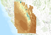
Future climates are simulated by general circulation models (GCM) using climate change scenarios (IPCC 2014). To project climate change for the sagebrush biome, we used 11 GCMs and two climate change scenarios from the IPCC Fifth Assessment, representative concentration pathways (RCPs) 4.5 and 8.5 (Moss et al. 2010, Van Vuuren et al. 2011). RCP4.5 scenario represents a future where climate policies limit and achieve stabilization of greenhouse gas concentrations to 4.5 W m-2 by 2100. RCP8.5 scenario might be called a business-as-usual scenario, where high emissions of greenhouse gases continue in the absence of climate change policies. The two selected time frames allow comparison of near-term (2020-2050) and longer-term...
Categories: Data;
Types: Citation,
Downloadable,
GeoTIFF,
Map Service,
Raster;
Tags: Arizona,
CRS,
California,
Climate,
Colorado,

This dataset is a Basin Characterization Model (BCM) output using the PCM A2 Scenario for annual recharge, 2010-2039, clipped to the DRECP 12 km buffered boundary. Recharge: Amount of water exceeding field capacity that enters bedrock, occurs at a rate determined by the hydraulic conductivity of the underlying materials, excess water (rejected recharge) is added to runoff. The California Basin Characterization Model (BCM) climate dataset provides historical and projected climate surfaces for the state at a 270 meter resolution. The historical data is based on 4 kilometer PRISM data, and the projected climate surfaces are based on the A2 and B1 scenarios of the PCM and GFDL GCMs. The BCM approach uses a regional...
This dataset is a Basin Characterization Model (BCM) output using the GFDL A2 Scenario for Climatic Water Deficit (CWD) in southern Sierra Nevada California, for 2010-2039. The term climatic water deficit defined by Stephenson (1998) is quantified as the amount of water by which potential evapotranspiration (PET) exceeds actual evapotranspiration (AET). This term effectively integrates the combined effects of solar radiation, evapotranspiration, and air temperature on watershed conditions given available soil moisture derived from precipitation. Climatic water deficit can be thought of as the amount of additional water that would have evaporated or transpired had it been present in the soils given the temperature...

This dataset is a Basin Characterization Model (BCM) output using the PCM A2 Scenario for annual Climatic Water Deficit (CWD), 2070-2099, clipped to the DRECP 12 km buffered boundary. The term climatic water deficit defined by Stephenson (1998) is quantified as the amount of water by which potential evapotranspiration (PET) exceeds actual evapotranspiration (AET). This term effectively integrates the combined effects of solar radiation, evapotranspiration, and air temperature on watershed conditions given available soil moisture derived from precipitation. Climatic water deficit can be thought of as the amount of additional water that would have evaporated or transpired had it been present in the soils given the...

This dataset is a Basin Characterization Model (BCM) output using the PCM A2 Scenario for average Spring (March, April, May) snowpack, in central Sierra Nevada California, for 2040-2069. Snowpack: Amount of snow accumulated per month summed annually, or if divided by 12 average monthly snowpack. This is calculated as prior month's snowpack plus snowfall minus sublimation and snow melt. The California Basin Characterization Model (BCM) climate dataset provides historical and projected climate surfaces for the state at a 270 meter resolution. The historical data is based on 4 kilometer PRISM data, and the projected climate surfaces are based on the A2 and B1 scenarios of the PCM and GFDL GCMs. The BCM approach uses...

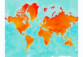
Using the simple anomaly method (modifying a historical baseline with differences or ratios projected by General Circulation Models), scientists from the California Academy of Sciences downscaled monthly average temperature and monthly total precipitation from 16 different global circulation models (GCMs). The GCMs were described in the latest Intergovernmental Panel for Climate Change (IPCC 2007) and archived at the WCRP PCMDI (http://www-pcmdi.llnl.gov/ipcc/about_ipcc.php). Monthly maximum temperature and monthly minimum temperatures were downscaled from the only 6 GCMs that archived these particular variables. Scientists used Worldclim v.1.4 (Hijmans et al 2005) at 5 arc-minute (~10km) spatial grain as the current...

Using the simple anomaly method (modifying a historical baseline with differences or ratios projected by General Circulation Models), scientists from the California Academy of Sciences downscaled monthly average temperature and monthly total precipitation from 16 different global circulation models (GCMs). The GCMs were described in the latest Intergovernmental Panel for Climate Change (IPCC 2007) and archived at the WCRP PCMDI (http://www-pcmdi.llnl.gov/ipcc/about_ipcc.php). Monthly maximum temperature and monthly minimum temperatures were downscaled from the only 6 GCMs that archived these particular variables. Scientists used Worldclim v.1.4 (Hijmans et al 2005) at 5 arc-minute (~10km) spatial grain as the current...

Using the simple anomaly method (modifying a historical baseline with differences or ratios projected by General Circulation Models), scientists from the California Academy of Sciences downscaled monthly average temperature and monthly total precipitation from 16 different global circulation models (GCMs). The GCMs were described in the latest Intergovernmental Panel for Climate Change (IPCC 2007) and archived at the WCRP PCMDI (http://www-pcmdi.llnl.gov/ipcc/about_ipcc.php). Monthly maximum temperature and monthly minimum temperatures were downscaled from the only 6 GCMs that archived these particular variables. Scientists used Worldclim v.1.4 (Hijmans et al 2005) at 5 arc-minute (~10km) spatial grain as the current...

Using the simple anomaly method (modifying a historical baseline with differences or ratios projected by General Circulation Models), scientists from the California Academy of Sciences downscaled monthly average temperature and monthly total precipitation from 16 different global circulation models (GCMs). The GCMs were described in the latest Intergovernmental Panel for Climate Change (IPCC 2007) and archived at the WCRP PCMDI (http://www-pcmdi.llnl.gov/ipcc/about_ipcc.php). Monthly maximum temperature and monthly minimum temperatures were downscaled from the only 6 GCMs that archived these particular variables. Scientists used Worldclim v.1.4 (Hijmans et al 2005) at 5 arc-minute (~10km) spatial grain as the current...
Using the simple anomaly method (modifying a historical baseline with differences or ratios projected by General Circulation Models), scientists from the California Academy of Sciences downscaled monthly average temperature and monthly total precipitation from 16 different global circulation models (GCMs). The GCMs were described in the latest Intergovernmental Panel for Climate Change (IPCC 2007) and archived at the WCRP PCMDI (http://www-pcmdi.llnl.gov/ipcc/about_ipcc.php). Monthly maximum temperature and monthly minimum temperatures were downscaled from the only 6 GCMs that archived these particular variables. Scientists used Worldclim v.1.4 (Hijmans et al 2005) at 5 arc-minute (~10km) spatial grain as the current...

Using the simple anomaly method (modifying a historical baseline with differences or ratios projected by General Circulation Models), scientists from the California Academy of Sciences downscaled monthly average temperature and monthly total precipitation from 16 different global circulation models (GCMs). The GCMs were described in the latest Intergovernmental Panel for Climate Change (IPCC 2007) and archived at the WCRP PCMDI (http://www-pcmdi.llnl.gov/ipcc/about_ipcc.php). Monthly maximum temperature and monthly minimum temperatures were downscaled from the only 6 GCMs that archived these particular variables. Scientists used Worldclim v.1.4 (Hijmans et al 2005) at 5 arc-minute (~10km) spatial grain as the current...

Using the simple anomaly method (modifying a historical baseline with differences or ratios projected by General Circulation Models), scientists from the California Academy of Sciences downscaled monthly average temperature and monthly total precipitation from 16 different global circulation models (GCMs). The GCMs were described in the latest Intergovernmental Panel for Climate Change (IPCC 2007) and archived at the WCRP PCMDI (http://www-pcmdi.llnl.gov/ipcc/about_ipcc.php). Monthly maximum temperature and monthly minimum temperatures were downscaled from the only 6 GCMs that archived these particular variables. Scientists used Worldclim v.1.4 (Hijmans et al 2005) at 5 arc-minute (~10km) spatial grain as the current...
|

|
